Physics Notes: String
Theory
Lecture 7: Nov 1, 2010 Back to PHY32
Topics: Fermion string oscillations, the analytic continuation trick for path integrals, action in string theories, surfaces of interaction, invariance under conformal mapping, applying conformal mapping to string scattering
Bosonic string theory (where the mass points are bosons) is not consistent because it contains a negative m2. In a normal QFT Hamiltonian such as

it is not possible to have negative energies because all
terms are positive, with a lowest energy (ground) state corresponding to a
constant ![]() .
.
If m2 = -1, then we have a disaster because the
energy continues to fall as ![]() increases
in magnitude.
increases
in magnitude.
A Fermionic string theory does not have the tachyon. These strings have two
kinds of oscillations.
One corresponds to oscillations in ![]() , the other to oscillations in spin or
, the other to oscillations in spin or ![]() . The x oscillations were
studied in previous lectures. The
spin oscillations arise from neighbor couplings of the spin of mass points.
. The x oscillations were
studied in previous lectures. The
spin oscillations arise from neighbor couplings of the spin of mass points.
Much like fermions contribution to the ground state in QFT,
these spin wave oscillations contribute negative energy of ![]() to
the ground state for each spin direction.
to
the ground state for each spin direction.
See: Vacuum Loops
This gives a way to have string states corresponding to photons and gravitons massless with out requiring m2=-1.
[There was a bit of discussion of
statistical mechanics here that I am leaving out. It may have a tie in to lecture 5, which I missed]
Fermionic string theory appears to be consistent and has a ground state.
The interaction Hamiltonian can be of two different forms:
![]() An antiferromagnet (opposite alignment is lowest energy)
An antiferromagnet (opposite alignment is lowest energy)
![]() A
ferromagnet (aligned
is lowest
A
ferromagnet (aligned
is lowest
energy)
In either case, if you disturb one mass point, spin waves propagate. Spin waves contribute negative energy.
Action in String Theory
We start with an ordinary particle moving from point x1 to x2. The path looks like:

We can compute the action for a free particle associated with the path as:
 Integrand
is the kinetic energy
Integrand
is the kinetic energy
To find the actual path taken we minimize S subject to the boundary condition that the path start and end with x1 and x2 .
In Quantum Mechanics the action has a different role. The action gives the phase for a
given path and we sum up over all possible paths to generate a propagator or
amplitude for the particles to start at x1 and end at x2.
![]()
In Feynman diagrams this amplitude is the propagator from vertex to vertex.

There is a problem with the integral. How does it converge? For any real S
![]() has
magnitude 1. We are counting
on a lot of cancellation. [Perhaps the
minimum path is defined by a kind of symmetry that for every deviation that
changes S by
has
magnitude 1. We are counting
on a lot of cancellation. [Perhaps the
minimum path is defined by a kind of symmetry that for every deviation that
changes S by ![]() ,
there is another deviation that changes S by
,
there is another deviation that changes S by ![]() .]
.]
There is a trick physicists use to evaluate path integrals. We start with a change of variables.
![]() Warning: this s is has nothing directly
to do with S.
Warning: this s is has nothing directly
to do with S.
Then the integral changes to:

The first ![]() comes with ds, the two on the bottom
come from the two derivatives in the integrand. Now we make the substitution.
comes with ds, the two on the bottom
come from the two derivatives in the integrand. Now we make the substitution.
![]()
Now

When we stick this into the integral over paths, the i’s cancel, leaving

[BTW – there is still a
problem with the measure for this integral. We need to parameterize the possible paths and figure out
a dp. I also seem to
remember a lattice model for summing the paths.]
In this form we see that excursions from the classical minimum
paths lead to large values of ![]() going out
and coming back, which reduces the contribution of paths fare away from the
minimum.
going out
and coming back, which reduces the contribution of paths fare away from the
minimum.
Now what you do is evaluate the integral between the s1 and s2, pretending that they are real. This leaves you with a function of s1 and s2. Then you chant analytic continuation three times before sticking in the complex values.
This is the only practical way to do path integrals.
[Need graph and paragraph on the contribution of excursions from the classical path].
Path Integrals in String Theory
We use the same kind of setup, but instead of a particle
path we have a world surface – a ribbon or a tube. You start by specifying ![]() at the
beginning and end.
at the
beginning and end.
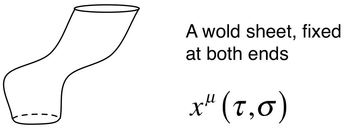
We make an action, which includes both the kinetic energy and the potential energy between mass points.

And similar to the case with paths, we sum across all surfaces connecting the starting configuration with the ending configuration.
![]()
Suppose you start with three closed strings and end with two. There are many alternate surfaces that are equally good. The two strings could combine before splitting three ways, or a first incoming string could split to connect to two of the outgoing strings with the remaining incoming string connecting to the remaining outgoing string. You can also have holes like the hole in a donut going through the world sheet.
This still has the convergence problem because all surfaces
contribute in the same way.
Again, we make the substitution ![]() and chant
analytic continuation.
and chant
analytic continuation.
Aside:
There are alternate forms of the action that yield the same physics. For particles, you can use the proper path length, and for strings, the area of the surface of the world sheet. This form is known as the Nambu-Gotu action.
Another action that is easier to calculate with is the Polyakov action. Susskind says that this action is really due to him, and that Polyakov invented another action which is called the Liouville action.
The substitution changes

into

Note: there could well be a missing ½ here from the Lagrangian.
If we had the first Lagrangian the equations of motion would be a standard wave equation. After the substitution we get a similar equation of motion
![]()
We see this equation in electrostatics in regions of space with no sources (the 0 on the right could be replaced by the source density).
We can recognize this as the Laplace equation. Suppose we pick a point in a
lattice with a spacing of ![]() .
.
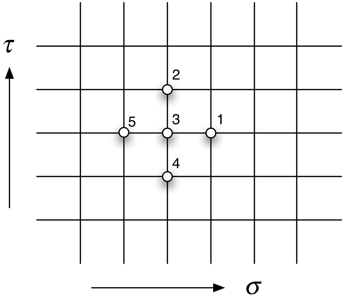
A first derivative in the ![]() direction
can be had by taking the difference in x at neighboring points:
direction
can be had by taking the difference in x at neighboring points:
![]()
Likewise, a first derivative in the ![]() direction would be
direction would be
![]()
Second derivatives are taken by taking differences between first derivatives, so
![]()
![]()
If we add these second derivatives up in both directions we must have 0 to satisfy the Laplace equation
![]()
Or
![]()
So the value of x at the center of a square must equal the average of the values at the corners. This is rotationally invariant.
What kinds of coordinate transforms preserve form of the Laplacian? If small squares are mapped to small squares, then the Laplacian won’t change.
The answer is conformal mapping. Conformal mappings preserve angles. This keeps the corners of the square in the right relative positions to each other. The area can expand or contract in the mapping.
It is possible to find conformal mappings between any two simple closed shapes. In the complex plane this corresponds to functions that are analytic (have non zero derivatives to all orders and are equal to their Taylor series).
There are issues with corners of shapes. Take the mapping of a square onto a rectangle. The corners of the square do not go to the obvious places in a conformal mapping.

Angle preservation fails at these points. [I suppose they become like point sources]. A corner in a shape is a place where the derivative of the tangent angle is discontinuous. In other places, if you zoom in far enough the curve looks like a straight line.
We can apply this conformal mapping to the model of two
strings joining and separating. In ![]() space we
had two strings joining for a period of time. We can map this space onto the unit circle.
space we
had two strings joining for a period of time. We can map this space onto the unit circle.
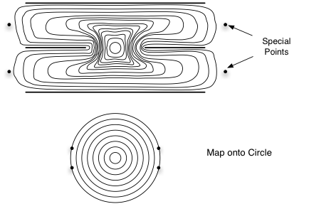
This mapping doesn’t change the form of the equation. The special points contain information about the incoming and outgoing particle states.
We have some freedom to specify the mapping. There is an overall rotation, which we can ignore. The important part of the mapping has to do with the location of the special, or injection points. It turns out that the time interval over which the strings are merged controls the spacing of the special points. If the time interval that the strings are joined is long, then the points are as I drew them, with the incoming points close together. If the time interval is short, then the point move to the top and bottom of the circle, placing one incoming/outgoing pair at the top and the other pair at the bottom. From this mapping onto a circle we can see a non-obvious symmetry between the S and T channels. See lecture 6.
This symmetry was called S-T duality and was discovered in 1969.